import numpy as np
import pandas as pd

# Plotly plotting support
import plotly.plotly as py
# import plotly.offline as py
# py.init_notebook_mode()

# import cufflinks as cf
# cf.go_offline() # required to use plotly offline (no account required).

import plotly.graph_objs as go
import plotly.figure_factory as ff

# Make the notebook deterministic
np.random.seed(42)
This notebook which accompanies the lecture on the Bias Variance Tradeoff and Regularization.
Notebook created by Joseph E. Gonzalez for DS100.
Introducing Regularization
In the previous notebook we adjusted the number of polynomial features to control model complexity and tradeoff bias and variance. However, this approach to managing model complexity has a few critical limitations:
- complexity varies discretely
- we may only need a few of the higher degree polynomial terms
- In general we may not have a natural way to order our basis
Rather than changing the dimension we can instead apply regularization to the weights. More generally, we can adopt the framework of regularized loss minimization.
$$ \large \hat{\theta} = \arg \min_\theta \frac{1}{n} \sum_{i=1}^n \textbf{Loss}\left(y_i, f_\theta(x_i)\right) + \lambda \textbf{R}(\theta) $$The regularization term $\textbf{R}(\theta)$ penalizes for $\theta$ values that result in more complex and therefore higher variance models. The regularization parameter $\lambda$ determines the degree of regularization to apply and is typically determined through cross validation.
Toy Dataset
As with the previous lectures we will continue to use an easy to visualize synthetic dataset.
np.random.seed(42)
n = 50
sigma = 10
X = np.linspace(-10, 10, n)
X = np.sort(X)
Y = 2. * X + 10. + sigma * np.random.randn(n) +  20*np.sin(X) + 0.8*(X)**2
X = X/5
data_points = go.Scatter(name="data", x=X, y=Y, mode='markers')
py.iplot([data_points])

## Train Test Split
from sklearn.model_selection import train_test_split
X_tr, X_te, Y_tr, Y_te = train_test_split(X, Y, test_size=0.25, random_state=42)
train_points = go.Scatter(name="Train Data",
                          x=X_tr, y=Y_tr, mode='markers',  marker=dict(color="blue", symbol="o"))
test_points = go.Scatter(name="Test Data",
                         x=X_te, y=Y_te, mode='markers', marker=dict(color="red", symbol="x"))
py.iplot([train_points, test_points], filename="toydataset-reg-lecture")
Polynomial Features:
Continuing from the previous lecture we will use polynomial features.
def poly_phi(k):
    return lambda X: np.array([np.sin(X*5)] + [X ** i for i in range(1, k+1)]).T
Ridge Regression
There are many forms for $\textbf{R}(\theta)$ but a common form is the squared $L^2$ norm of $\theta$.
$$\large \large \textbf{R}_{L^2}(\theta) = \large||\theta||_2^2 = \theta^T \theta = \sum_{k=1}^p \theta_k^2 $$In the context of least squares regression this is often referred to as Ridge Regression with the objective:
$$ \large \hat{\theta} = \arg \min_\theta \frac{1}{n} \sum_{i=1}^n \left(y_i - f_\theta(x_i)\right)^2 + \lambda ||\theta||_2^2 $$This is also sometimes called Tikhonov Regularization.
Deriving the optimal $\hat{\theta}$ with $L^2$ Regularization
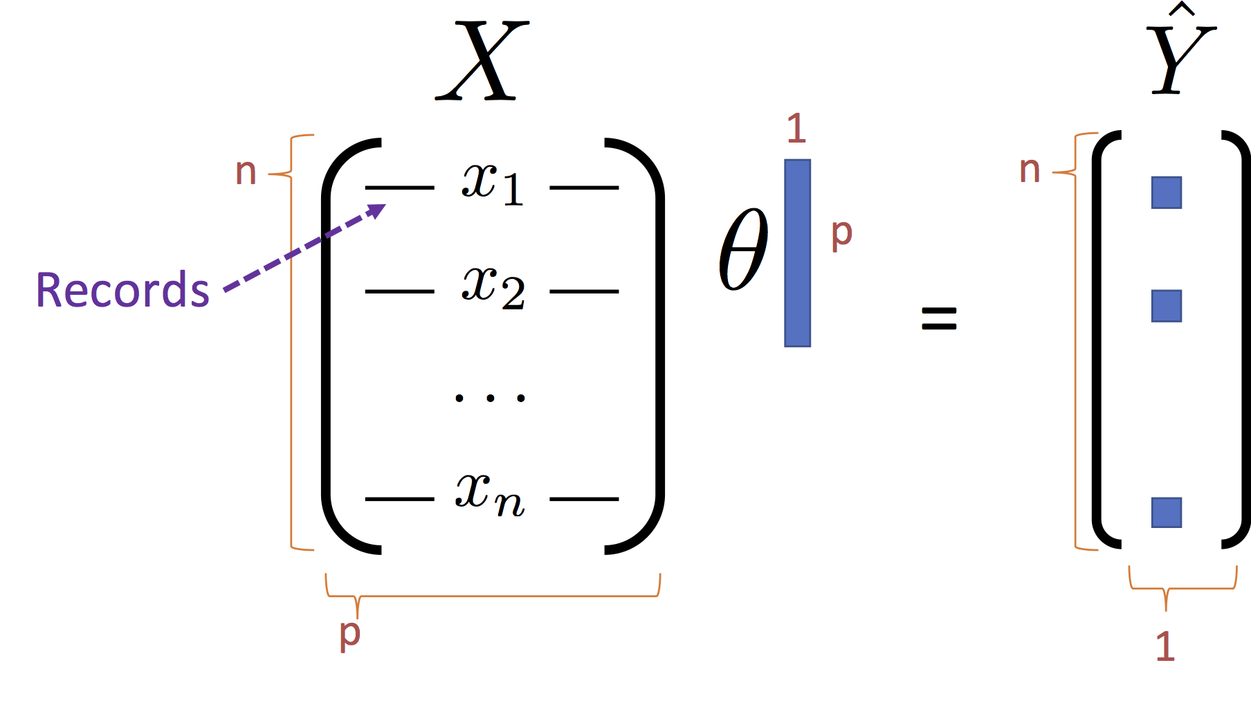
We return to our linear model formulation:
$$ \large f_\theta(x) = x^T \theta $$Using the standard matrix notation:
We can rewrite the objection
\begin{align}\large \hat{\theta}_{\text{L2}} = \arg\min_\theta \frac{1}{n}\left(Y - X \theta \right)^T \left(Y - X \theta \right) + \lambda \theta^T \theta \end{align}Expanding the objective term:
\begin{align}\large L_\lambda(\theta) = \left(Y - X \theta \right)^T \left(Y - X \theta \right) + \lambda \theta^T \theta = \frac{1}{n} \left( Y^T Y - 2 Y^T X \theta + \theta^T X^T X \theta \right) + \lambda \theta^T \theta \end{align}Taking the gradient with respect to $\theta$:
\begin{align} \large \nabla_\theta L_\lambda(\theta) & \large = \frac{1}{n} \left( \nabla_\theta Y^T Y - \nabla_\theta 2 Y^T X \theta + \nabla_\theta \theta^T X^T X \theta \right) + \nabla_\theta \lambda \theta^T \theta \\ & \large = \frac{1}{n} \left( 0 - 2 X^T Y + 2 X^T X \theta \right) + 2\lambda \theta \end{align}The above gradient derivation uses the following identities:
- $\large \nabla_\theta \left( A \theta \right) = A^T$
- $\large \nabla_\theta \left( \theta^T A \theta \right) = A\theta + A^T \theta$ and $\large A = X^T X$ is symmetric
Setting the gradient equal to zero we get a regularized version of the normal equations:
$$\large (X^T X + n \lambda I) \theta = X^T Y $$$$\large \theta = \left(X^T X + n \lambda I \right)^{-1} X^T Y $$Optimal $\theta$ under $L^2$ regularization
Because $\lambda$ is a tuning parameter we often will absorb the $n$ into $\lambda$ and rewrite the above equations as:
$$\large (X^T X + \lambda I) \theta = X^T Y $$$$\large \theta = \left(X^T X + \lambda I \right)^{-1} X^T Y $$Notice: The addition of $\lambda I$ ensures that $X^T X + \lambda I$ is full rank. This addresses the earlier issue in least-squares regression when we had co-linear features.
How does $L^2$ Regularization Help
The $L^2$ penalty helps in several ways:
Manages Model Complexity
- It ensures that uninformative features weights are relatively small (near zero) mitigating the affect of those features.
- It evenly distributes weight over similar features to reduce variance.
Practical Concerns
- It removes degeneracy created by co-linear features
- It improves the numerical stability of
Visualizing $L^2$ Regularization
In the following we visualize the regularization surface. Notice that it pushes weights towards zero but is relatively smooth around the origin.
theta_range = np.linspace(-2,2,100)
(u,v) = np.meshgrid(theta_range, theta_range)
w_values = np.vstack((u.flatten(), v.flatten())).T

def l2_sq_reg(w):
    return np.sum(w**2)
reg_values = [l2_sq_reg(w) for w in w_values]
reg_surface = go.Surface(
    x = u, y = v,
    z = np.reshape(reg_values, u.shape),
    contours=dict(z=dict(show=True))
)

# Axis labels
layout = go.Layout(
    scene=go.Scene(
        xaxis=go.XAxis(title='w0'),
        yaxis=go.YAxis(title='w1'),
        aspectratio=dict(x=2.,y=2., z=1.),
        camera=dict(eye=dict(x=-2, y=-2, z=2))
    )
)
fig = go.Figure(data = [reg_surface], layout = layout)
py.iplot(fig, filename="L2regularization")
Applying $L^2$ Regularization using Scikit Learn
In the following we use the linear_model.Ridge model in scikit learn. To demonstrate the efficacy of regularization we will use the degree 32 polynomials which substantially overfit the data.
Phi = poly_phi(32)(X_tr)
Normalization and the Intercept
Before we proceed it is important that we appropriately normalize the data. Because the standard $L^2$ regularization methods treat each dimensional equivalently it is important that all dimensions are in the same range of values.
However, if we examine the polynomial features in $\Phi$ we notice that the distribution of values can be quite different for each dimension.
For example in the following we plot the degree 3 and degree 6 dimensions:
py.iplot(ff.create_distplot([Phi[:,3], Phi[:,6]], group_labels=['x^3', 'x^6']), filename="phi_dist_plot")
Notice:
- difference in spread
- asymmetry
Standardizing the Data
A common transformation is to center and scale the features to zero mean and unit variance:
$$\large z = \frac{x - \mu}{\sigma} $$This an be accomplished by applying the StandardScalar scikit learn preprocessor.
from sklearn.preprocessing import StandardScaler

normalizer = StandardScaler()
normalizer.fit(poly_phi(32)(X_tr))
# we define the phi function for reuse in the future
def phi_fun(X):
    return normalizer.transform(poly_phi(32)(X))

Phi = phi_fun(X_tr)
Notice in the above code snippet we define a new $\Phi$ function that applies the pre-trained normalization. This procedure learns something about the training data in the formulation of the normalizer.
- Will this be an issue when we cross validate on the training data?
This process of transformations: feature construction, rescaling, and then subsequently model fitting form pipelines. Scikit learn actually has a pipeline framework to aid with this process.
In the following we plot the spread of the transformed dimensions. They are still not the same but are at least on the same scale.
py.iplot(ff.create_distplot([Phi[:,3], Phi[:,6]], group_labels=['x^4', 'x^7'], bin_size=0.3), filename="phi_dist_plot2")
Fitting the Ridge Regression Model
We are now finally ready to fit the ridge regression model. However, we haven't yet decided on a value for the regularization parameter $\lambda$. Therefore, we will try a range of values.
import sklearn.linear_model as linear_model
lam_values = np.hstack((np.logspace(-8,-1,10), np.logspace(-1,2,10),np.logspace(2,10,10)))

models = [
    linear_model.Ridge(alpha = lam).fit(Phi, Y_tr)
    for lam in lam_values
]

#     model = linear_model.Ridge(alpha = lam)
#     model.fit(Phi, Y_tr)
#     models.append(model)
Move the slider in the following plot to see the fit for various $\lambda$ values.
# Make the x values where plot points will be generated
X_plt = np.linspace(np.min(X)-1, np.max(X)+1, 200)

# Generate the Plotly line objects by predicting the value at each X_plt
lines = []
for k in range(len(models)):
    ytmp = models[k].predict(phi_fun(X_plt))
    # Plotting software fails with large numbers
    ytmp[ytmp > 500] = 500
    ytmp[ytmp < -500] = -500
    lines.append(
        go.Scatter(name="Lambda "+ str(lam_values[k]),
                   x=X_plt, y = ytmp, visible=False))

# Construct steps for the interactive slider
lines[0].visible=True
steps = []
for i in range(len(lines)):
    step = dict(
        label = lines[i]['name'],
        method = 'restyle',
        args = ['visible', [False] * (len(lines)+1)],
    )
    step['args'][1][0] = True
    step['args'][1][i+1] = True # Toggle i'th trace to "visible"
    steps.append(step)

# Build the slider object
sliders = [dict(active = 0, pad = {"t": 20}, steps = steps)]

# render the plot
layout = go.Layout(xaxis=dict(range=[np.min(X_plt), np.max(X_plt)]),
                   yaxis=dict(range=[np.min(Y) -5 , np.max(Y) + 5]),
                   sliders=sliders,
                   showlegend=False)
py.iplot(go.Figure(data = [train_points] + lines, layout=layout), filename="ridge_regression_lines")
For large $\lambda$ values we see a smoother fit. Notice however that the model does not appear to perform well outside of the input data range. This is a common problem with polynomial feature transformations.
Using Cross Validation in the RidgeCV Model
Because cross validation is essential to determining the optimal regularization parameter there is built-in support for cross validation in linear_model.RidgeCV. Here we call the built-in cross validation routine passing the lambda values we wish to consider.
ridge_cv_model = linear_model.RidgeCV(alphas=lam_values, store_cv_values=True)
# Fit the model to our training data
ridge_cv_model.fit(Phi, Y_tr)

# Plot the predicted model
ridge_cv_line = go.Scatter(name = "Ridge CV Curve",
                           x = X_plt,
                           y = ridge_cv_model.predict(phi_fun(X_plt)))
# render the plot
layout = go.Layout(xaxis=dict(range=[np.min(X_plt), np.max(X_plt)]),
                   yaxis=dict(range=[np.min(Y) -5 , np.max(Y)+5]))
py.iplot(go.Figure(data = [train_points, ridge_cv_line], layout=layout), filename="ridge_cv_line")
ridge_cv_loss = np.sqrt(np.mean(ridge_cv_model.cv_values_,axis=0))
py.iplot(
    go.Figure(
        data=[go.Scatter(name="CV Curve", x=lam_values, y=ridge_cv_loss),
              go.Scatter(name="Optimum", x=[lam_values[np.argmin(ridge_cv_loss)]], y=[np.min(ridge_cv_loss)],
                         mode="markers", marker=dict(color="red", size=10))
             ],
        layout=go.Layout(xaxis=dict(title="Lambda", type="log"),
                         yaxis=dict(title="CV RMSE", range=[10,70]))),
    filename="ridge_cv_model_curve")
Question: What is going on with small $\lambda$ values?
$L^1$ Regularization (Lasso)
Another common regularization function is the sum of the absolute values:
$$\large \large \textbf{R}_{L^1}(\theta) = \sum_{k=1}^p |\theta_k| $$This is called $L^1$ regularization as it corresponds to the $L^1$ norm. Least squares linear regression in conjunction with the $L^1$ norm is often called the Lasso (Least Absolute Shrinkage and Selection Operator).
In contrast to the $L^2$ norm the $L^1$ norm encourages $\theta_i$ values to be exactly zero in less informative dimensions thereby reducing model complexity. To see how the $L^1$ encourages sparsity consider the following illustration:
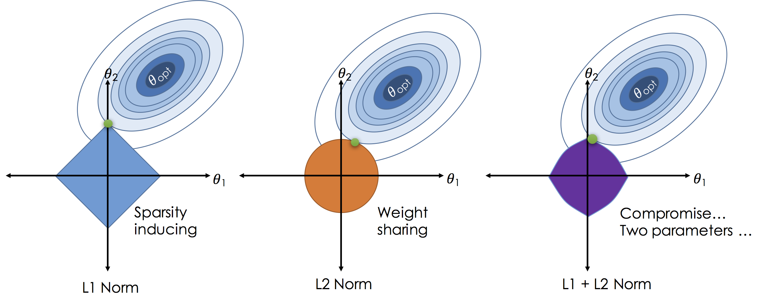
In the above figures we plot the loss for settings of a two dimensional ($\theta_1$ and $\theta_2$) model as the elliptical contours. Without regularization the solution would be at the center of the contours. By imposing regularization we constrain the solution to living in the "norm ball" centered at the origin (all zero theta vector). As we increase $\lambda$ we actually shrink the ball. Unlike the $L^2$ solutions in the $L^1$ will often "slide to the corners" which are aligned with axis causing subsets of the $\theta$ vector to be exactly zero.
In some settings a compromise can be achieved by using both the $L^2$ and $L^1$ norms to encourage sparsity while ensuring relatively co-linear features are given equal weight (to improve robustness).
theta_range = np.linspace(-2,2,100)
(u,v) = np.meshgrid(theta_range, theta_range)
w_values = np.vstack((u.flatten(), v.flatten())).T

def l1_reg(w):
    return np.sum(np.abs(w))
reg_values = [l1_reg(w) for w in w_values]
reg_surface = go.Surface(
    x = u, y = v,
    z = np.reshape(reg_values, u.shape),
    contours=dict(z=dict(show=True))
)

# Axis labels
layout = go.Layout(
    scene=go.Scene(
        xaxis=go.XAxis(title='w0'),
        yaxis=go.YAxis(title='w1'),
        aspectratio=dict(x=2.,y=2., z=1.),
        camera=dict(eye=dict(x=-2, y=-2, z=2))
    )
)
fig = go.Figure(data = [reg_surface], layout = layout)
py.iplot(fig, filename="L1regularization")
$L^1$ regularized regression in scikit-learn
In the following we use the scikit-learn Lasso package. As before we will try a range of values for the regularization parameter.
lam_values = np.logspace(-1.3,2.5,20)
models = []
for lam in lam_values:
    model = linear_model.Lasso(alpha = lam, max_iter=100000)
    model.fit(Phi, Y_tr)
    models.append(model)
Again we can plot the fit for different regularization penalties.
# Make the x values where plot points will be generated
X_plt = np.linspace(np.min(X)-1, np.max(X)+1, 200)

# Generate the Plotly line objects by predicting the value at each X_plt
lines = []
# Make the full polynomial
poly = np.array([r"\theta_0 \sin(x)"] + [r" \theta_{" + str(d) + "} x^{"+str(d)+"} " for d in range(1, 33)])


for k in range(len(models)):
    ytmp = models[k].predict(phi_fun(X_plt))
    # Plotting software fails with large numbers
    ytmp[ytmp > 500] = 500
    ytmp[ytmp < -500] = -500
    num_features = np.sum(~np.isclose(models[k].coef_, 0.))
    # get all the nonzer terms
    #     non_zero_terms = ~np.isclose(models[k].coef_,0)
    #     poly_str = "$" +("+".join(poly[non_zero_terms])) + "$"
    lines.append(
        go.Scatter(name=(
            "Lambda "+ str(lam_values[k]) +
            " num features = " + str(num_features)
            + " out of " + str(len(models[k].coef_))),
                   x=X_plt, y = ytmp, visible=False))

# Construct steps for the interactive slider
lines[0].visible=True
steps = []
for i in range(len(lines)):
    step = dict(
        label = lines[i]['name'],
        method = 'restyle',
        args = ['visible', [False] * (len(lines)+1)],
    )
    step['args'][1][0] = True
    step['args'][1][i+1] = True # Toggle i'th trace to "visible"
    steps.append(step)

# Build the slider object
sliders = [dict(active = 0, pad = {"t": 20}, steps = steps)]

# render the plot
layout = go.Layout(xaxis=dict(range=[np.min(X_plt), np.max(X_plt)]),
                   yaxis=dict(range=[np.min(Y) -5 , np.max(Y) + 5]),
                   sliders=sliders,
                   showlegend=False)
py.iplot(go.Figure(data = [train_points] + lines, layout=layout), filename="lasso_regression_lines")
Cross Validated Solution
As with Ridge regression, scikit-learn provides support for cross validation directly in the Lasso model training procedure. In the following we LassoCV to determine the best regularization parameter.
lasso_cv_model = linear_model.LassoCV(alphas=lam_values, max_iter=1000000)
# Fit the model to our training data
lasso_cv_model.fit(Phi, Y_tr)

# Plot the predicted model
lasso_cv_line = go.Scatter(name = "Lasso CV Curve",
                           x = X_plt,
                           y = lasso_cv_model.predict(phi_fun(X_plt)))
# render the plot
layout = go.Layout(xaxis=dict(range=[np.min(X_plt), np.max(X_plt)]),
                   yaxis=dict(range=[np.min(Y) -5 , np.max(Y)+5]))
py.iplot(go.Figure(data = [train_points, lasso_cv_line], layout=layout), filename="lasso_cv_line")
Let's look at the polynomial terms with non-zero $\theta$
from IPython.display import display, Markdown

# get all the nonzer terms
non_zero_terms = ~np.isclose(lasso_cv_model.coef_,0)

# Make the full polynomial
poly = np.array([r"\theta_0 \sin(x)"] + [r" \theta_{" + str(d) + "} x^{"+str(d)+"} " for d in range(1, 33)])

# Print only the nonzero terms
display(Markdown(r"$\large" + ("+".join(poly[non_zero_terms])) + "$"))
from sklearn.metrics import mean_squared_error
from sklearn.model_selection import KFold


kfold_splits = 5
kfold = KFold(kfold_splits, shuffle=True, random_state=42)

mse_scores = []
for lam in lam_values:
    # One step in k-fold cross validation
    def score_model(train_index, test_index):
        model = linear_model.Lasso(alpha=lam, max_iter=1000000)
        model.fit(Phi[train_index,:], Y_tr[train_index])
        return mean_squared_error(Y_tr[test_index], model.predict(Phi[test_index,]))

    mse_score = np.mean([score_model(tr_ind, te_ind)
                     for (tr_ind, te_ind) in kfold.split(Phi)])
    mse_scores.append(mse_score)
rmse_scores = np.sqrt(np.array(mse_scores))


py.iplot(
    go.Figure(
        data=[go.Scatter(name="CV Curve", x=lam_values, y=rmse_scores),
              go.Scatter(name="Optimum", x=[lam_values[np.argmin(rmse_scores)]], y=[np.min(rmse_scores)],
                         mode="markers", marker=dict(color="red", size=10))
             ],
        layout=go.Layout(xaxis=dict(title="Lambda",type="log",range=[-1.2,1.5]),
                         yaxis=dict(title="CV RMSE", range=[5,30]))),
    filename="lasso_cv_model_curve")